38 excel graph data labels different series
Comparison Chart in Excel | Adding Multiple Series Under Same Graph Please note that there is no such option as Comparison Chart under Excel to proceed with. We just have added a bar/column chart with multiple series values (2018 and 2019). However, adding two series under the same graph makes it automatically look like a comparison since each series values have a separate bar/column associated with it. 3 Axis Graph Excel Method: Add a Third Y-Axis - EngineerExcel Next, I added a fourth data series to create the 3 axis graph in Excel. The x-values for the series were the array of constants and the y-values were the unscaled values. I also modified the line style to match the weight of the other gridlines, added markers (the kind that look like plus signs), and changed the color of the line and marker to ...
Dynamically Label Excel Chart Series Lines - My Online Training … Sep 26, 2017 · The Label Series Data contains a formula that only returns the value for the last row of data. You can see in the image below that the formula in cell G5 is: =IF(AND(C6="",C5<>""), [@[UK Data]],NA()) As new data is added the formula dynamically fills down because my data is formatted in an Excel Table , hence the [@[UK Data]] structured ...
Excel graph data labels different series
How to Make a Bar Graph in Excel: 9 Steps (with Pictures) - wikiHow 02/05/2022 · It's easy to spruce up data in Excel and make it easier to interpret by converting it to a bar graph. A bar graph is not only quick to see and understand, but it's also more engaging than a list of numbers. ... Add labels for the graph's X- and Y-axes. To do so, click the A1 cell (X-axis) ... This will select all of your data. If your graph ... Find, label and highlight a certain data point in Excel scatter graph Oct 10, 2018 · Add a new data series for the data point. With the source data ready, let's create a data point spotter. For this, we will have to add a new data series to our Excel scatter chart: Right-click any axis in your chart and click Select Data…. In the Select Data Source dialogue box, click the Add button. In the Edit Series window, do the following: How to add a line in Excel graph: average line, benchmark, etc. 12/09/2018 · Tips: The same technique can be used to plot a median For this, use the MEDIAN function instead of AVERAGE.; Adding a target line or benchmark line in your graph is even simpler. Instead of a formula, enter your target values in the last column and insert the Clustered Column - Line combo chart as shown in this example.; If none of the predefined combo charts …
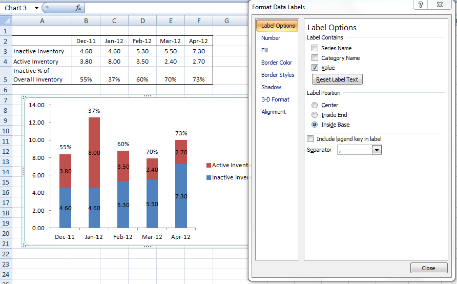
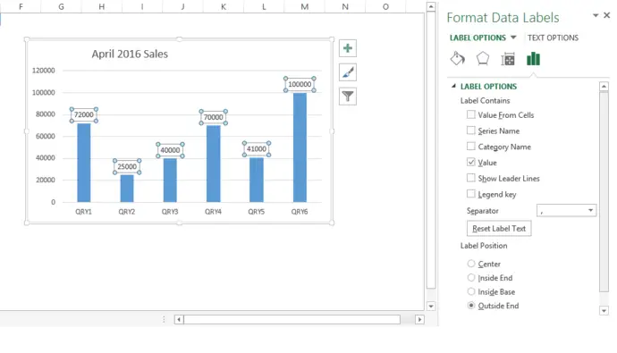
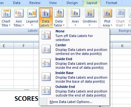
Excel graph data labels different series. How to add data labels from different column in an Excel chart? This method will introduce a solution to add all data labels from a different column in an Excel chart at the same time. Please do as follows: 1. Right click the data series in the chart, and select Add Data Labels > Add Data Labels from the context menu to add data labels. 2. Right click the data series, and select Format Data Labels from the ... Create Dynamic Chart Data Labels with Slicers - Excel Campus 10/02/2016 · Step 3: Use the TEXT Function to Format the Labels. Typically a chart will display data labels based on the underlying source data for the chart. In Excel 2013 a new feature called “Value from Cells” was introduced. This feature allows us to specify the a range that we want to use for the labels. Prevent Overlapping Data Labels in Excel Charts - Peltier Tech May 24, 2021 · I recently wrote a post called Slope Chart with Data Labels which provided a simple VBA procedure to add data labels to a slope chart; the procedure simplified the problem caused by positioning each data label individually for each point in the chart. The problem is that often points are located close to each other; the result: overlapping data ... How to Change Excel Chart Data Labels to Custom Values? - Chandoo.org May 05, 2010 · First add data labels to the chart (Layout Ribbon > Data Labels) Define the new data label values in a bunch of cells, like this: Now, click on any data label. This will select “all” data labels. Now click once again. At this point excel will select only one data label.
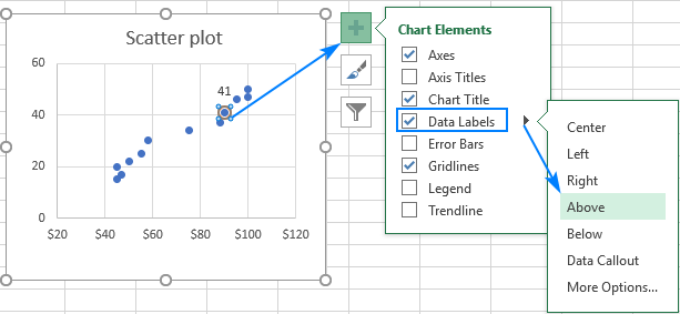
How to add a line in Excel graph: average line, benchmark, etc. 12/09/2018 · Tips: The same technique can be used to plot a median For this, use the MEDIAN function instead of AVERAGE.; Adding a target line or benchmark line in your graph is even simpler. Instead of a formula, enter your target values in the last column and insert the Clustered Column - Line combo chart as shown in this example.; If none of the predefined combo charts … Find, label and highlight a certain data point in Excel scatter graph Oct 10, 2018 · Add a new data series for the data point. With the source data ready, let's create a data point spotter. For this, we will have to add a new data series to our Excel scatter chart: Right-click any axis in your chart and click Select Data…. In the Select Data Source dialogue box, click the Add button. In the Edit Series window, do the following: How to Make a Bar Graph in Excel: 9 Steps (with Pictures) - wikiHow 02/05/2022 · It's easy to spruce up data in Excel and make it easier to interpret by converting it to a bar graph. A bar graph is not only quick to see and understand, but it's also more engaging than a list of numbers. ... Add labels for the graph's X- and Y-axes. To do so, click the A1 cell (X-axis) ... This will select all of your data. If your graph ...
30 How To Label Points In Excel - Labels For You

How to Import, Graph, and Label Excel Data in MATLAB: 13 Steps

Advanced Graphs Using Excel : create line plot with error bar plot in excel

Multiple bar charts on one axis in excel - Super User
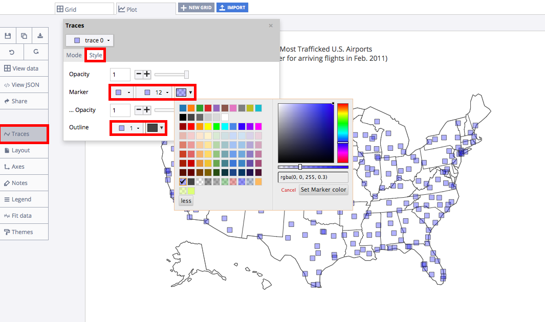
Make a Scatter Plot on a Map with Chart Studio and Excel
November 2018
35 How To Label Bar Graph In Excel - Best Labeling Ideas
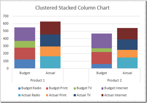
How-to Make an Excel Clustered Stacked Column Chart with Different Colors by Stack - Excel ...
31 How To Label Graph In Excel - Labels Database 2020
Excel-labeling everything in a graph with talking software - YouTube

How to Make Pie Charts and Graphs in Excel - BSUPERIOR

Programmatically adding excel data labels in a bar chart - Stack Overflow

How to add data labels from different column in an Excel chart?
How To Create 3 Axis Chart In Excel - best excel tutorial 3 axis chartgraphically displaying ...
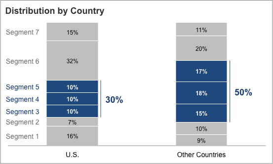
How-to Put Percentage Labels on Top of a Stacked Column Chart - Excel Dashboard Templates

highcharts - Optimal display for overlapping series in a line chart - Stack Overflow
Formula Friday - Using Formulas To Add Custom Data Labels To Your Excel Chart - How To Excel At ...
how to make a excel graph.
Post a Comment for "38 excel graph data labels different series"